Predicting Boston Housing Prices : Exploratory Data Analysis (EDA)

The Boston Housing dataset is one of the classic beginner projects in machine learning. I worked on this as part of my learning journey and wanted to share a few key steps that I personally found interesting or worth paying attention to.
This isn’t meant to be a full tutorial — instead, I’ll walk through the main parts of the process that stood out to me: how we test relationships between features, apply log transformations, evaluate model fit using BIC, and use RMSE to build a prediction range.
Along the way, I’ll also be trying out a few different ways to visualize the results — mostly just to explore more plotting options and get better at using them. These variations aren’t necessary to follow, but they all use the same core functions and are good for practice.
The idea is to keep things simple and practical. If you’re also exploring ML and want to build intuition for how regression works in real datasets, I hope this post helps you spot the “why” behind some of the steps — not just the code itself.
This project was part of my learning journey, not a tutorial.
Load the Boston Housing Dataset from URL
The dataset is fetched directly from Carnegie Mellon University’s open data repository.
The file format is unusual — every data sample spans two rows:
- The first row has 12 features
- The second row has the remaining 2 features + the target value (housing price)
We use:
read_csv()with a custom separator (\\s+) to handle whitespaceskiprows=22to skip the descriptive headernp.hstack()to horizontally stack every pair of rows:- the 1st, 3rd, 5th rows for features
- the 2nd, 4th, 6th rows for extra features and target
- We extract the third column from every second row as the target variable (
target)
This preprocessing reconstructs the dataset into a proper format where each row represents one complete data point.
1
2
3
4
5
data_url = "http://lib.stat.cmu.edu/datasets/boston"
raw_df = pd.read_csv(data_url, sep="\\s+", skiprows=22, header=None)
data = np.hstack([raw_df.values[::2, :], raw_df.values[1::2, :2]])
target = raw_df.values[1::2, 2]
Verify Data Structure After Reconstruction
After combining rows using
np.hstack, we check the shape and content of our dataset:
data.shapeconfirms that we now have 506 rows and 13 columns, meaning 506 complete data points (each with 13 features).data[0]prints the first data sample, helping us visually inspect that the reconstruction worked correctly and values are aligned.
This step is crucial for validating that our reshaping logic hasn’t misaligned any features or rows — a silent bug here could break all downstream analysis.
1
2
print(data.shape)
print(data[0])
1
2
3
(506, 13)
[6.320e-03 1.800e+01 2.310e+00 0.000e+00 5.380e-01 6.575e+00 6.520e+01
 4.090e+00 1.000e+00 2.960e+02 1.530e+01 3.969e+02 4.980e+00]
1
2
3
4
5
6
7
8
9
10
11
12
13
14
15
16
features = [
    "CRIM",     # per capita crime rate by town
    "ZN",       # proportion of residential land zoned for lots over 25,000 sq.ft.
    "INDUS",    # proportion of non-retail business acres per town
    "CHAS",     # Charles River dummy variable (= 1 if tract bounds river; 0 otherwise)
    "NOX",      # nitric oxides concentration (parts per 10 million)
    "RM",       # average number of rooms per dwelling
    "AGE",      # proportion of owner-occupied units built prior to 1940
    "DIS",      # weighted distances to five Boston employment centres
    "RAD",      # index of accessibility to radial highways
    "TAX",      # full-value property-tax rate per $10,000
    "PTRATIO",  # pupil-teacher ratio by town
    "B",        # 1000(Bk - 0.63)^2 where Bk is the proportion of Black residents by town
    "LSTAT"     # % lower status of the population
]
1
2
3
data= pd.DataFrame(data= data , columns= features)
data["PRICE"] = target
print(data)
1
2
3
4
5
6
7
8
9
10
11
12
13
14
        CRIM    ZN  INDUS  CHAS    NOX  ...    TAX  PTRATIO       B  LSTAT  PRICE
0    0.00632  18.0   2.31   0.0  0.538  ...  296.0     15.3  396.90   4.98   24.0
1    0.02731   0.0   7.07   0.0  0.469  ...  242.0     17.8  396.90   9.14   21.6
2    0.02729   0.0   7.07   0.0  0.469  ...  242.0     17.8  392.83   4.03   34.7
3    0.03237   0.0   2.18   0.0  0.458  ...  222.0     18.7  394.63   2.94   33.4
4    0.06905   0.0   2.18   0.0  0.458  ...  222.0     18.7  396.90   5.33   36.2
..       ...   ...    ...   ...    ...  ...    ...      ...     ...    ...    ...
501  0.06263   0.0  11.93   0.0  0.573  ...  273.0     21.0  391.99   9.67   22.4
502  0.04527   0.0  11.93   0.0  0.573  ...  273.0     21.0  396.90   9.08   20.6
503  0.06076   0.0  11.93   0.0  0.573  ...  273.0     21.0  396.90   5.64   23.9
504  0.10959   0.0  11.93   0.0  0.573  ...  273.0     21.0  393.45   6.48   22.0
505  0.04741   0.0  11.93   0.0  0.573  ...  273.0     21.0  396.90   7.88   11.9

[506 rows x 14 columns]
1
data.tail()
| CRIM | ZN | INDUS | CHAS | NOX | RM | AGE | DIS | RAD | TAX | PTRATIO | B | LSTAT | PRICE | |
|---|---|---|---|---|---|---|---|---|---|---|---|---|---|---|
| 501 | 0.06263 | 0.0 | 11.93 | 0.0 | 0.573 | 6.593 | 69.1 | 2.4786 | 1.0 | 273.0 | 21.0 | 391.99 | 9.67 | 22.4 |
| 502 | 0.04527 | 0.0 | 11.93 | 0.0 | 0.573 | 6.120 | 76.7 | 2.2875 | 1.0 | 273.0 | 21.0 | 396.90 | 9.08 | 20.6 |
| 503 | 0.06076 | 0.0 | 11.93 | 0.0 | 0.573 | 6.976 | 91.0 | 2.1675 | 1.0 | 273.0 | 21.0 | 396.90 | 5.64 | 23.9 |
| 504 | 0.10959 | 0.0 | 11.93 | 0.0 | 0.573 | 6.794 | 89.3 | 2.3889 | 1.0 | 273.0 | 21.0 | 393.45 | 6.48 | 22.0 |
| 505 | 0.04741 | 0.0 | 11.93 | 0.0 | 0.573 | 6.030 | 80.8 | 2.5050 | 1.0 | 273.0 | 21.0 | 396.90 | 7.88 | 11.9 |
1
data.info()
1
2
3
4
5
6
7
8
9
10
11
12
13
14
15
16
17
18
19
20
21
<class 'pandas.core.frame.DataFrame'>
RangeIndex: 506 entries, 0 to 505
Data columns (total 14 columns):
 #   Column   Non-Null Count  Dtype
---  ------   --------------  -----
 0   CRIM     506 non-null    float64
 1   ZN       506 non-null    float64
 2   INDUS    506 non-null    float64
 3   CHAS     506 non-null    float64
 4   NOX      506 non-null    float64
 5   RM       506 non-null    float64
 6   AGE      506 non-null    float64
 7   DIS      506 non-null    float64
 8   RAD      506 non-null    float64
 9   TAX      506 non-null    float64
 10  PTRATIO  506 non-null    float64
 11  B        506 non-null    float64
 12  LSTAT    506 non-null    float64
 13  PRICE    506 non-null    float64
dtypes: float64(14)
memory usage: 55.5 KB
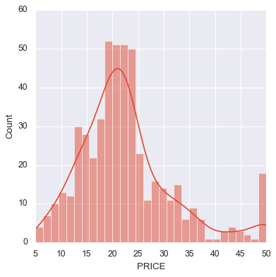
Visualize the Distribution of Housing Prices
Before modeling, it’s helpful to understand the distribution of the target variable — in this case,
PRICE(in $1000s).
We plot a histogram with:
bins=30for smoother granularity- a clean visual style (
tealcolor, black edges, slight transparency) - labeled axes for readability
This plot helps us see:
- Whether the target is normally distributed
- If there are outliers or skew (e.g., a long tail to the right)
- Whether we might need to apply a transformation (like log) later
Note: If you’re getting an error like
TypeError: 'numpy.ndarray' object is not subscriptable, make suredatais a DataFrame, not a NumPy array, before plotting.
1
2
sb.displot(data.PRICE,bins=30,kde=True)
# sb.displot(data.PRICE)
1
data.describe()
| CRIM | ZN | INDUS | CHAS | NOX | RM | AGE | DIS | RAD | TAX | PTRATIO | B | LSTAT | PRICE | |
|---|---|---|---|---|---|---|---|---|---|---|---|---|---|---|
| count | 506.000000 | 506.000000 | 506.000000 | 506.000000 | 506.000000 | 506.000000 | 506.000000 | 506.000000 | 506.000000 | 506.000000 | 506.000000 | 506.000000 | 506.000000 | 506.000000 |
| mean | 3.613524 | 11.363636 | 11.136779 | 0.069170 | 0.554695 | 6.284634 | 68.574901 | 3.795043 | 9.549407 | 408.237154 | 18.455534 | 356.674032 | 12.653063 | 22.532806 |
| std | 8.601545 | 23.322453 | 6.860353 | 0.253994 | 0.115878 | 0.702617 | 28.148861 | 2.105710 | 8.707259 | 168.537116 | 2.164946 | 91.294864 | 7.141062 | 9.197104 |
| min | 0.006320 | 0.000000 | 0.460000 | 0.000000 | 0.385000 | 3.561000 | 2.900000 | 1.129600 | 1.000000 | 187.000000 | 12.600000 | 0.320000 | 1.730000 | 5.000000 |
| 25% | 0.082045 | 0.000000 | 5.190000 | 0.000000 | 0.449000 | 5.885500 | 45.025000 | 2.100175 | 4.000000 | 279.000000 | 17.400000 | 375.377500 | 6.950000 | 17.025000 |
| 50% | 0.256510 | 0.000000 | 9.690000 | 0.000000 | 0.538000 | 6.208500 | 77.500000 | 3.207450 | 5.000000 | 330.000000 | 19.050000 | 391.440000 | 11.360000 | 21.200000 |
| 75% | 3.677083 | 12.500000 | 18.100000 | 0.000000 | 0.624000 | 6.623500 | 94.075000 | 5.188425 | 24.000000 | 666.000000 | 20.200000 | 396.225000 | 16.955000 | 25.000000 |
| max | 88.976200 | 100.000000 | 27.740000 | 1.000000 | 0.871000 | 8.780000 | 100.000000 | 12.126500 | 24.000000 | 711.000000 | 22.000000 | 396.900000 | 37.970000 | 50.000000 |
1
2
3
4
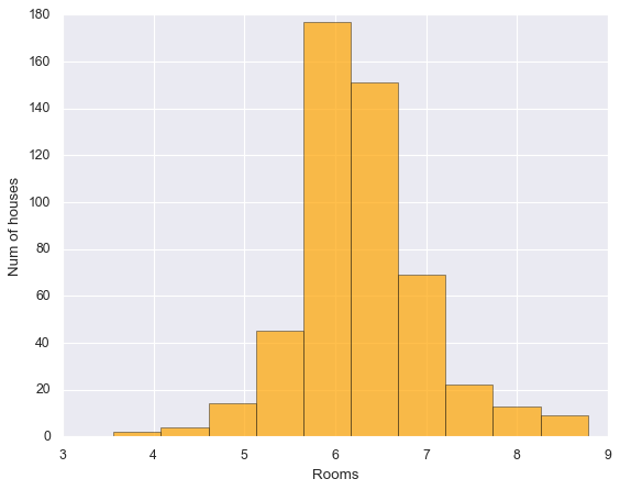
plt.Figure(figsize=(12,8))
plt.hist(data["RM"],bins=10, color = "orange", edgecolor="black", alpha=0.7 )
plt.xlabel("Rooms", fontsize = 12)
plt.ylabel("Num of houses",fontsize = 12)
Check Linear Correlation Between Features and Target
We loop through each feature and calculate its Pearson correlation with
PRICE.
- Pearson correlation ranges from -1 to 1:
+1: perfect positive linear relationship-1: perfect negative linear relationship0: no linear relationship
- This helps us identify features that are strongly correlated with the target — useful for linear regression.
Features with high positive or negative correlation to
PRICEmay be strong predictors.
This step also gives us a quick numeric intuition of which features are likely to be useful in the model and which may not contribute much.
1
data.corr()
| CRIM | ZN | INDUS | CHAS | NOX | RM | AGE | DIS | RAD | TAX | PTRATIO | B | LSTAT | PRICE | |
|---|---|---|---|---|---|---|---|---|---|---|---|---|---|---|
| CRIM | 1.000000 | -0.200469 | 0.406583 | -0.055892 | 0.420972 | -0.219247 | 0.352734 | -0.379670 | 0.625505 | 0.582764 | 0.289946 | -0.385064 | 0.455621 | -0.388305 |
| ZN | -0.200469 | 1.000000 | -0.533828 | -0.042697 | -0.516604 | 0.311991 | -0.569537 | 0.664408 | -0.311948 | -0.314563 | -0.391679 | 0.175520 | -0.412995 | 0.360445 |
| INDUS | 0.406583 | -0.533828 | 1.000000 | 0.062938 | 0.763651 | -0.391676 | 0.644779 | -0.708027 | 0.595129 | 0.720760 | 0.383248 | -0.356977 | 0.603800 | -0.483725 |
| CHAS | -0.055892 | -0.042697 | 0.062938 | 1.000000 | 0.091203 | 0.091251 | 0.086518 | -0.099176 | -0.007368 | -0.035587 | -0.121515 | 0.048788 | -0.053929 | 0.175260 |
| NOX | 0.420972 | -0.516604 | 0.763651 | 0.091203 | 1.000000 | -0.302188 | 0.731470 | -0.769230 | 0.611441 | 0.668023 | 0.188933 | -0.380051 | 0.590879 | -0.427321 |
| RM | -0.219247 | 0.311991 | -0.391676 | 0.091251 | -0.302188 | 1.000000 | -0.240265 | 0.205246 | -0.209847 | -0.292048 | -0.355501 | 0.128069 | -0.613808 | 0.695360 |
| AGE | 0.352734 | -0.569537 | 0.644779 | 0.086518 | 0.731470 | -0.240265 | 1.000000 | -0.747881 | 0.456022 | 0.506456 | 0.261515 | -0.273534 | 0.602339 | -0.376955 |
| DIS | -0.379670 | 0.664408 | -0.708027 | -0.099176 | -0.769230 | 0.205246 | -0.747881 | 1.000000 | -0.494588 | -0.534432 | -0.232471 | 0.291512 | -0.496996 | 0.249929 |
| RAD | 0.625505 | -0.311948 | 0.595129 | -0.007368 | 0.611441 | -0.209847 | 0.456022 | -0.494588 | 1.000000 | 0.910228 | 0.464741 | -0.444413 | 0.488676 | -0.381626 |
| TAX | 0.582764 | -0.314563 | 0.720760 | -0.035587 | 0.668023 | -0.292048 | 0.506456 | -0.534432 | 0.910228 | 1.000000 | 0.460853 | -0.441808 | 0.543993 | -0.468536 |
| PTRATIO | 0.289946 | -0.391679 | 0.383248 | -0.121515 | 0.188933 | -0.355501 | 0.261515 | -0.232471 | 0.464741 | 0.460853 | 1.000000 | -0.177383 | 0.374044 | -0.507787 |
| B | -0.385064 | 0.175520 | -0.356977 | 0.048788 | -0.380051 | 0.128069 | -0.273534 | 0.291512 | -0.444413 | -0.441808 | -0.177383 | 1.000000 | -0.366087 | 0.333461 |
| LSTAT | 0.455621 | -0.412995 | 0.603800 | -0.053929 | 0.590879 | -0.613808 | 0.602339 | -0.496996 | 0.488676 | 0.543993 | 0.374044 | -0.366087 | 1.000000 | -0.737663 |
| PRICE | -0.388305 | 0.360445 | -0.483725 | 0.175260 | -0.427321 | 0.695360 | -0.376955 | 0.249929 | -0.381626 | -0.468536 | -0.507787 | 0.333461 | -0.737663 | 1.000000 |
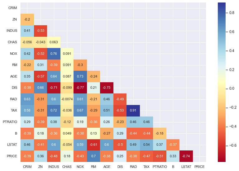
Create a Triangular Mask for Correlation Heatmap
To visualize the feature–feature correlations, we’ll later use a heatmap. Since correlation matrices are symmetrical, we mask one triangle to avoid redundancy.
What’s happening here:
data.corr()generates the full correlation matrix.np.zeros_like(...)creates a matrix of zeros with the same shape.np.triu_indices_from(mask)gets the indices of the upper triangle.- We set the upper triangle values in
masktoTrueso they get hidden in the heatmap.
This keeps the plot clean and focused by only showing one half of the matrix.
1
2
3
4
5
6
mask = np.zeros_like(data.corr())
triangle_indices = np.triu_indices_from(mask)
# triangle_indices

mask[triangle_indices] = True
mask
1
2
3
4
5
6
7
8
9
10
11
12
13
14
array([[1., 1., 1., 1., 1., 1., 1., 1., 1., 1., 1., 1., 1., 1.],
       [0., 1., 1., 1., 1., 1., 1., 1., 1., 1., 1., 1., 1., 1.],
       [0., 0., 1., 1., 1., 1., 1., 1., 1., 1., 1., 1., 1., 1.],
       [0., 0., 0., 1., 1., 1., 1., 1., 1., 1., 1., 1., 1., 1.],
       [0., 0., 0., 0., 1., 1., 1., 1., 1., 1., 1., 1., 1., 1.],
       [0., 0., 0., 0., 0., 1., 1., 1., 1., 1., 1., 1., 1., 1.],
       [0., 0., 0., 0., 0., 0., 1., 1., 1., 1., 1., 1., 1., 1.],
       [0., 0., 0., 0., 0., 0., 0., 1., 1., 1., 1., 1., 1., 1.],
       [0., 0., 0., 0., 0., 0., 0., 0., 1., 1., 1., 1., 1., 1.],
       [0., 0., 0., 0., 0., 0., 0., 0., 0., 1., 1., 1., 1., 1.],
       [0., 0., 0., 0., 0., 0., 0., 0., 0., 0., 1., 1., 1., 1.],
       [0., 0., 0., 0., 0., 0., 0., 0., 0., 0., 0., 1., 1., 1.],
       [0., 0., 0., 0., 0., 0., 0., 0., 0., 0., 0., 0., 1., 1.],
       [0., 0., 0., 0., 0., 0., 0., 0., 0., 0., 0., 0., 0., 1.]])
1
2
3
4
5
plt.figure(figsize=(12,8))
sb.heatmap(data.corr(), mask=mask, cmap= "RdYlBu" , annot=True)
sb.set_style("dark")
plt.xticks(fontsize=10)
plt.yticks(fontsize=10)
1
2
3
4
5
6
7
8
9
10
11
12
13
14
15
16
(array([ 0.5,  1.5,  2.5,  3.5,  4.5,  5.5,  6.5,  7.5,  8.5,  9.5, 10.5,
        11.5, 12.5, 13.5]),
 [Text(0, 0.5, 'CRIM'),
  Text(0, 1.5, 'ZN'),
  Text(0, 2.5, 'INDUS'),
  Text(0, 3.5, 'CHAS'),
  Text(0, 4.5, 'NOX'),
  Text(0, 5.5, 'RM'),
  Text(0, 6.5, 'AGE'),
  Text(0, 7.5, 'DIS'),
  Text(0, 8.5, 'RAD'),
  Text(0, 9.5, 'TAX'),
  Text(0, 10.5, 'PTRATIO'),
  Text(0, 11.5, 'B'),
  Text(0, 12.5, 'LSTAT'),
  Text(0, 13.5, 'PRICE')])
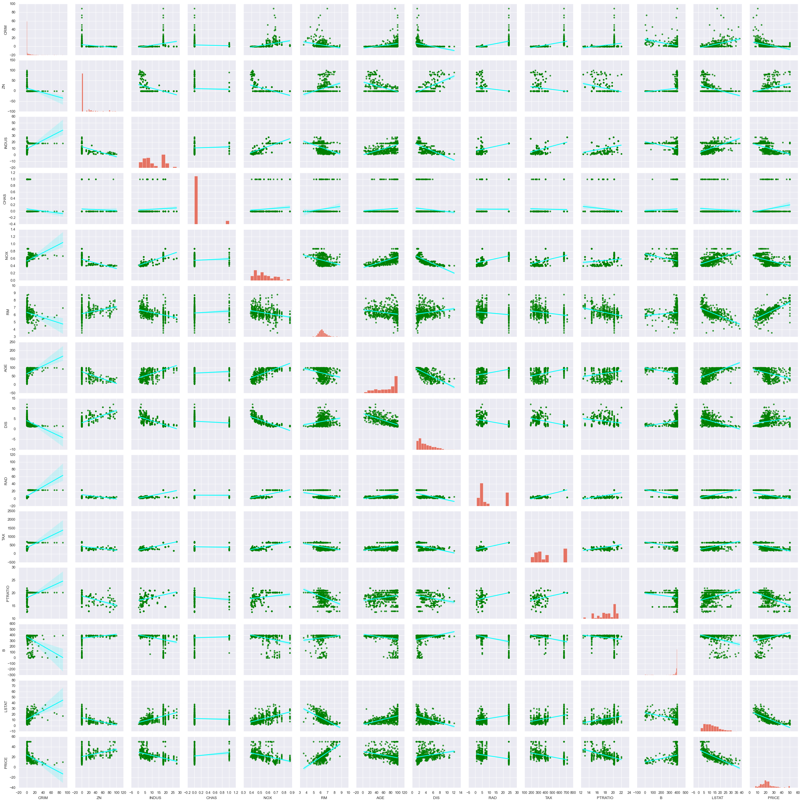
1
sb.pairplot(data, kind = "reg", plot_kws= {'line_kws':{'color':'cyan'}, 'scatter_kws':{'color':'green'}})
1
<seaborn.axisgrid.PairGrid at 0x17ef21ed0>
Separate Features and Target Variable
We now split the dataset into:
features: all independent variables (used for prediction)prices: the target variable we’re trying to predict —PRICE
We use drop("PRICE", axis=1) to remove the target column from the feature set.
This separation is important for:
- Supervised learning models, which require a clear input (X) and output (y)
- Later steps like scaling, fitting, and evaluation
At this point,
featurescontains all predictors andpricescontains the house prices in $1000s.
1
2
prices = data.PRICE
features = data.drop("PRICE", axis = 1)     #### to remove a col off
Multivariable Linear Regression Overview
In multivariable linear regression, we try to predict the target variable (
PRICE) as a weighted sum of all input features, plus an intercept.
The general form of the equation looks like this:
\[\hat{\text{Price}} = \theta_0 + \theta_1 \cdot \text{RM} + \theta_2 \cdot \text{NOX} + \cdots + \theta_n \cdot N\]Where:
- $\theta_0$ is the intercept — the baseline prediction when all features are zero
- $\theta_1, \theta_2, \dots, \theta_n$ are the coefficients learned by the model
RM,NOX, …,Nare the actual input features from the dataset- The coefficient $\theta_1$ controls the weight of the
RMfeature
These $\theta$ values (coefficients) are what the model “learns” during training. The intercept stays fixed for a given model, but the individual feature weights can change depending on which features we include or exclude.
This is the underlying formula estimated when we use LinearRegression().fit() or statsmodels.OLS().
Splitting the Data: Train vs Test Sets
To evaluate model performance fairly, we split our dataset into:
x_train,y_train: used to train the model (80% of data)x_test,y_test: used to test generalization (20% of data)
We use train_test_split() from sklearn.model_selection, with:
test_size=0.2→ 20% of the data goes to the test setrandom_state=10→ makes the split reproducible
This step helps us check whether our model performs well on unseen data and isn’t just memorizing patterns from training.
1
x_train,x_test,y_train,y_test = tts(features,prices,test_size=0.2,random_state=10)
Fit a Linear Regression Model
We create a
LinearRegressionobject and fit it to the training data using.fit(x_train, y_train).
This step estimates:
- the intercept (baseline value)
- the coefficients (weights for each feature)
These learned parameters define the multivariable regression equation used to predict house prices.
The second
regr_test = LR()is likely for a later use on the test set (e.g., predicting and evaluating).
1
2
3
regr = LR()
regr_test = LR()
regr.fit(x_train,y_train)
1
2
print(regr.intercept_)
trained_coef = pd.DataFrame(data = regr.coef_, index= x_train.columns , columns=["Coefficient"])
1
36.53305138282447
1
2
trained_coef
| Feature | Coefficient |
|---|---|
| CRIM | -0.128181 |
| ZN | 0.063198 |
| INDUS | -0.007576 |
| CHAS | 1.974515 |
| NOX | -16.271989 |
| RM | 3.108456 |
| AGE | 0.016292 |
| DIS | -1.483014 |
| RAD | 0.303988 |
| TAX | -0.012082 |
| PTRATIO | -0.820306 |
| B | 0.011419 |
| LSTAT | -0.581626 |
Evaluate Model Using R² Score
We assess how well our trained model performs using the coefficient of determination (R² score), calculated with
.score().
R²measures the proportion of variance in the target variable explained by the features.- Ranges from 0 to 1:
1means perfect prediction0means the model does no better than the mean
We compute:
r2_train: model performance on the training setr2_test: performance on unseen test data
In this case:
- Training R² = 0.75 → decent fit to the training data
- Testing R² = 0.67 → slightly lower, indicating some generalization loss but no extreme overfitting
R² gives a quick and interpretable snapshot of how well our model is capturing the underlying pattern in the data.
1
2
3
4
r2_test = regr.score(x_test,y_test)
r2_train = regr.score(x_train,y_train)
print(f"R2 for test data: {regr.score(x_test,y_test)}")
print(f"R2 for trained data: {regr.score(x_train,y_train)}")
1
2
R2 for test data: 0.6709339839115636
R2 for trained data: 0.750121534530608
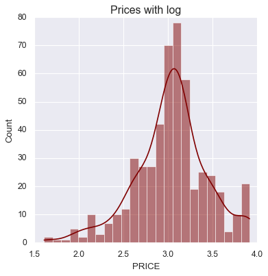
Check Skewness and Apply Log Transformation
We compute the skewness of the target variable (
PRICE) to assess its distribution.
- Skewness tells us how asymmetric the data is:
0= perfectly symmetric (normal)- Positive skew = long right tail (common with price/income data)
In this case:
prices.skew()returns ≈ 1.11, meaning right-skewed- Right-skewed data can distort regression assumptions
To address this, we apply a log transformation using
np.log(), which compresses large values and reduces skew.
This improves linearity, stabilizes variance, and makes the model more statistically sound.
1
prices.skew()
1
np.float64(1.1080984082549072)
1
2
prices_log = np.log(data.PRICE)
prices_log.skew()
1
np.float64(-0.33032129530987864)
1
2
sb.displot(prices_log, color="maroon", kde=True)
plt.title("Prices with log")
1
Text(0.5, 1.0, 'Prices with log')
Train Regression Model on Log-Transformed Prices
After reducing skewness in
PRICEusing a log transformation, we re-train the model to better meet linear regression assumptions.
We repeat the steps:
- Apply
train_test_split()to split features and log-transformed target - Initialize a new
LinearRegressionobject - Fit the model on training data using
.fit(x_train, y_train)
Using the log of
PRICEhelps:
- Make the relationship between features and target more linear
- Normalize residuals
- Improve interpretability for percentage-based effects
This model is now predicting log(price), not raw price. We’ll exponentiate the predictions later to return to original dollar units.
1
2
3
4
prices_log = np.log(data.PRICE)
x_train,x_test,y_train,y_test= tts(features , prices_log, random_state=10, test_size= 0.2)
log_reg = LR()
log_reg.fit(x_train,y_train)
1
pd.DataFrame(columns=["Coeff"], data=log_reg.coef_, index=features.columns)
| Coeff | |
|---|---|
| CRIM | -0.010672 |
| ZN | 0.001579 |
| INDUS | 0.002030 |
| CHAS | 0.080331 |
| NOX | -0.704068 |
| RM | 0.073404 |
| AGE | 0.000763 |
| DIS | -0.047633 |
| RAD | 0.014565 |
| TAX | -0.000645 |
| PTRATIO | -0.034795 |
| B | 0.000516 |
| LSTAT | -0.031390 |
1
print(f"Intercept : {log_reg.intercept_}")
1
Intercept : 4.059943871775207
1
2
print(f"R2 value of Trained set : {log_reg.score(x_train,y_train)}")
print(f"R2 value of Test set : {log_reg.score(x_test,y_test)}")
1
2
R2 value of Trained set : 0.7930234826697584
R2 value of Test set : 0.7446922306260739
P values and evaluating Coeffs
1
2
3
4
5
x_incl_const = sm.add_constant(x_train)

model = sm.OLS(y_train,x_incl_const)

results = model.fit()
1
pd.DataFrame({"Coef":results.params, "Pvalues":round(results.pvalues,3)})
| Coef | Pvalues | |
|---|---|---|
| const | 4.059944 | 0.000 |
| CRIM | -0.010672 | 0.000 |
| ZN | 0.001579 | 0.009 |
| INDUS | 0.002030 | 0.445 |
| CHAS | 0.080331 | 0.038 |
| NOX | -0.704068 | 0.000 |
| RM | 0.073404 | 0.000 |
| AGE | 0.000763 | 0.209 |
| DIS | -0.047633 | 0.000 |
| RAD | 0.014565 | 0.000 |
| TAX | -0.000645 | 0.000 |
| PTRATIO | -0.034795 | 0.000 |
| B | 0.000516 | 0.000 |
| LSTAT | -0.031390 | 0.000 |
1
results.rsquared
1
np.float64(0.7930234826697584)
Testing for Multicollinearity with VIF
Multicollinearity happens when two or more input features are strongly correlated with each other. This can make the model’s coefficient estimates unreliable or overly sensitive to small changes in the data.
We test for this using VIF (Variance Inflation Factor), which measures how much the variance of a regression coefficient is inflated due to multicollinearity.
The formula for VIF is:
\[\text{VIF}_i = \frac{1}{1 - R^2_i}\]Where:
- $R^2_i$ is the coefficient of determination when the i-th feature is regressed against all the other features.
🔍 How to interpret VIF:
- VIF ≈ 1 → No multicollinearity
- VIF = 1–5 → Generally acceptable
- VIF = 5–10 → Moderate correlation, may need checking
- VIF > 10 → Strong multicollinearity — consider removing the feature
By calculating VIF scores for all features, we can identify which ones may be redundant and remove them to improve both the stability and interpretability of the model.
1
2
3
4
5
6
7
# VIF = vif(exog = x_incl_const.values ,exog_idx=13 )
# VIF
vif_list  = []
for i in range(1,len(x_incl_const.columns)):
    VIF =  vif(exog= x_incl_const.values,exog_idx= i )
    vif_list.append(VIF)
vif_list
1
2
3
4
5
6
7
8
9
10
11
12
13
[np.float64(1.714525044393249),
 np.float64(2.3328224265597597),
 np.float64(3.943448822674638),
 np.float64(1.0788133385000576),
 np.float64(4.410320817897634),
 np.float64(1.8404053075678568),
 np.float64(3.3267660823099394),
 np.float64(4.222923410477865),
 np.float64(7.314299817005058),
 np.float64(8.508856493040817),
 np.float64(1.8399116326514058),
 np.float64(1.338671325536472),
 np.float64(2.812544292793035)]
1
2
type(x_incl_const)
type(x_incl_const.values)
1
numpy.ndarray
1
len(x_incl_const.columns)
1
14
1
2
vif_list  = [ vif(exog= x_incl_const.values,exog_idx= i) for i in range(1,len(x_incl_const.columns) ) ]
vif_list
1
2
3
4
5
6
7
8
9
10
11
12
13
[np.float64(1.714525044393249),
 np.float64(2.3328224265597597),
 np.float64(3.943448822674638),
 np.float64(1.0788133385000576),
 np.float64(4.410320817897634),
 np.float64(1.8404053075678568),
 np.float64(3.3267660823099394),
 np.float64(4.222923410477865),
 np.float64(7.314299817005058),
 np.float64(8.508856493040817),
 np.float64(1.8399116326514058),
 np.float64(1.338671325536472),
 np.float64(2.812544292793035)]
1
pd.DataFrame({"coef_name": features.columns,"VIF":vif_list} )
| index | coef_name | VIF |
|---|---|---|
| 0 | CRIM | 1.714525 |
| 1 | ZN | 2.332822 |
| 2 | INDUS | 3.943449 |
| 3 | CHAS | 1.078813 |
| 4 | NOX | 4.410321 |
| 5 | RM | 1.840405 |
| 6 | AGE | 3.326766 |
| 7 | DIS | 4.222923 |
| 8 | RAD | 7.314300 |
| 9 | TAX | 8.508856 |
| 10 | PTRATIO | 1.839912 |
| 11 | B | 1.338671 |
| 12 | LSTAT | 2.812544 |
Model Simplification Using Bayesian Information Criterion (BIC)
Once we have several candidate models, we use Bayesian Information Criterion (BIC) to compare them.
BIC helps us balance:
- Model fit (how well the model explains the data)
- Model complexity (how many features are used)
The key idea:
- Lower BIC = better model
- BIC penalizes models with more features, discouraging overfitting
We may try simplified versions of the model by:
- Removing weak or redundant features (like
INDUSandAGE) - Re-fitting the model
- Selecting the version with the lowest BIC
This ensures the model generalizes better while staying interpretable.
1
results.summary()
| Dep. Variable: | PRICE | R-squared: | 0.793 |
|---|---|---|---|
| Model: | OLS | Adj. R-squared: | 0.786 |
| Method: | Least Squares | F-statistic: | 114.9 |
| Date: | Mon, 26 May 2025 | Prob (F-statistic): | 1.70e-124 |
| Time: | 05:17:07 | Log-Likelihood: | 111.88 |
| No. Observations: | 404 | AIC: | -195.8 |
| Df Residuals: | 390 | BIC: | -139.7 |
| Df Model: | 13 | ||
| Covariance Type: | nonrobust |
| coef | std err | t | P>|t| | [0.025 | 0.975] | |
|---|---|---|---|---|---|---|
| const | 4.0599 | 0.227 | 17.880 | 0.000 | 3.614 | 4.506 |
| CRIM | -0.0107 | 0.001 | -7.971 | 0.000 | -0.013 | -0.008 |
| ZN | 0.0016 | 0.001 | 2.641 | 0.009 | 0.000 | 0.003 |
| INDUS | 0.0020 | 0.003 | 0.765 | 0.445 | -0.003 | 0.007 |
| CHAS | 0.0803 | 0.039 | 2.079 | 0.038 | 0.004 | 0.156 |
| NOX | -0.7041 | 0.166 | -4.245 | 0.000 | -1.030 | -0.378 |
| RM | 0.0734 | 0.019 | 3.910 | 0.000 | 0.036 | 0.110 |
| AGE | 0.0008 | 0.001 | 1.258 | 0.209 | -0.000 | 0.002 |
| DIS | -0.0476 | 0.009 | -5.313 | 0.000 | -0.065 | -0.030 |
| RAD | 0.0146 | 0.003 | 5.170 | 0.000 | 0.009 | 0.020 |
| TAX | -0.0006 | 0.000 | -4.095 | 0.000 | -0.001 | -0.000 |
| PTRATIO | -0.0348 | 0.006 | -5.908 | 0.000 | -0.046 | -0.023 |
| B | 0.0005 | 0.000 | 4.578 | 0.000 | 0.000 | 0.001 |
| LSTAT | -0.0314 | 0.002 | -14.213 | 0.000 | -0.036 | -0.027 |
| Omnibus: | 28.711 | Durbin-Watson: | 2.059 |
|---|---|---|---|
| Prob(Omnibus): | 0.000 | Jarque-Bera (JB): | 105.952 |
| Skew: | 0.093 | Prob(JB): | 9.84e-24 |
| Kurtosis: | 5.502 | Cond. No. | 1.54e+04 |
Notes:
[1] Standard Errors assume that the covariance matrix of the errors is correctly specified.
[2] The condition number is large, 1.54e+04. This might indicate that there are
strong multicollinearity or other numerical problems.
Simplifying the Model with BIC and R²
To improve model generalization and interpretability, we simplify the regression model by removing less important features and evaluating each version using:
- BIC (Bayesian Information Criterion) — lower is better
- R² (explained variance) — higher is better
Model 2: Removed INDUS
- Dropping
INDUSled to:- BIC = -145.145
- R² = 0.793
- This indicates a good balance between simplicity and predictive power.
Model 3: Removed INDUS and AGE
- Further removed
AGEto reduce complexity - Reran the regression and compared results
By iteratively dropping features and comparing metrics, we choose the version with the lowest BIC that still maintains strong explanatory performance.
This step helps us lock in a minimal yet effective feature set before final residual checks and predictions.
1
2
3
4
5
6
7
##Model 1
x_incl_const = sm.add_constant(x_train)
model_1 = sm.OLS(y_train,x_incl_const)
result_1 = model_1.fit()
model_1 = pd.DataFrame({"Coef":result_1.params, "Pvalues":round(result_1.pvalues,3)})
print(f"BIC: {round(result_1.bic,3)}")
print(f"Rsquared : {round(result_1.rsquared,3)}")
1
2
BIC: -139.75
Rsquared : 0.793
1
2
3
4
5
6
7
8
#Model 2 without INDUS
x_incl_const = sm.add_constant(x_train)
x_incl_const =x_incl_const.drop(["INDUS"],axis=1)
model_2 = sm.OLS(y_train,x_incl_const)
result_2 = model_2.fit()
model_2 = pd.DataFrame({"Coef":result_2.params, "Pvalues":round(result_2.pvalues,3)})
print(f"BIC: {round(result_2.bic,3)}")
print(f"Rsquared : {round(result_2.rsquared,3)}")
1
2
BIC: -145.145
Rsquared : 0.793
1
2
3
4
5
6
7
8
#Model 3 without INDUS & AGE
x_incl_const = sm.add_constant(x_train)
x_incl_const =x_incl_const.drop(["INDUS","AGE"],axis=1)
model_3 = sm.OLS(y_train,x_incl_const)
result_3 = model_3.fit()
model_3 = pd.DataFrame({"Coef":result_3.params, "Pvalues":round(result_3.pvalues,3)})
print(f"BIC: {round(result_3.bic,3)}")
print(f"Rsquared : {round(result_3.rsquared,3)}")
1
2
BIC: -149.499
Rsquared : 0.792
1
2
models_list = [model_1,model_2,model_3]
pd.concat(models_list, axis = 1)
| Feature | Coef | Pvalues | Coef | Pvalues | Coef | Pvalues |
|---|---|---|---|---|---|---|
| const | 4.059944 | 0.000 | 4.056231 | 0.000 | 4.035922 | 0.000 |
| CRIM | -0.010672 | 0.000 | -0.010721 | 0.000 | -0.010702 | 0.000 |
| ZN | 0.001579 | 0.009 | 0.001551 | 0.010 | 0.001461 | 0.014 |
| INDUS | 0.002030 | 0.445 | NaN | NaN | NaN | NaN |
| CHAS | 0.080331 | 0.038 | 0.082795 | 0.032 | 0.086449 | 0.025 |
| NOX | -0.704068 | 0.000 | -0.673365 | 0.000 | -0.616448 | 0.000 |
| RM | 0.073404 | 0.000 | 0.071739 | 0.000 | 0.076133 | 0.000 |
| AGE | 0.000763 | 0.209 | 0.000766 | 0.207 | NaN | NaN |
| DIS | -0.047633 | 0.000 | -0.049394 | 0.000 | -0.052692 | 0.000 |
| RAD | 0.014565 | 0.000 | 0.014014 | 0.000 | 0.013743 | 0.000 |
| TAX | -0.000645 | 0.000 | -0.000596 | 0.000 | -0.000590 | 0.000 |
| PTRATIO | -0.034795 | 0.000 | -0.034126 | 0.000 | -0.033481 | 0.000 |
| B | 0.000516 | 0.000 | 0.000511 | 0.000 | 0.000518 | 0.000 |
| LSTAT | -0.031390 | 0.000 | -0.031262 | 0.000 | -0.030271 | 0.000 |
Residuals and plots
1
2
3
4
5
6
7
8
9
10
11
12
13
14
15
16
### Latest model
prices_log = np.log(data.PRICE)

# features = features.drop(["AGE","INDUS"], axis = 1)
x_train,x_test,y_train,y_test= tts(features , prices_log, random_state=10, test_size= 0.2)
log_reg = LR()
log_reg.fit(x_train,y_train)
x_incl_const = sm.add_constant(x_train)

# x_incl_const =x_incl_const.drop(["INDUS","AGE"],axis=1)
model_x = sm.OLS(y_train,x_incl_const)
result_x = model_x.fit()
model_x = pd.DataFrame({"Coef":result_x.params, "Pvalues":round(result_x.pvalues,3)})

print(f"BIC: {round(result_x.bic,3)}")
print(f"Rsquared : {round(result_x.rsquared,3)}")
1
2
BIC: -149.499
Rsquared : 0.792
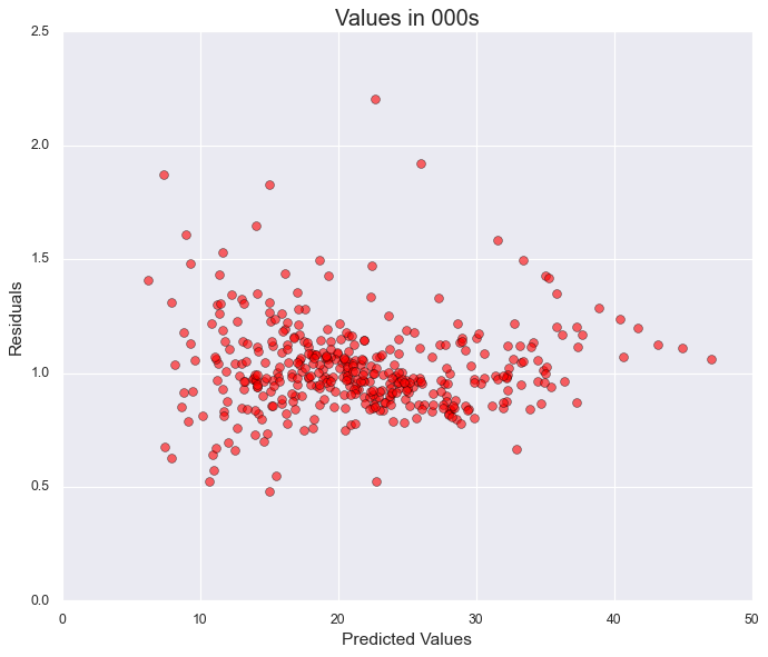
Residual Analysis and Model Diagnostics
After finalizing our simplified regression model, we perform residual analysis to verify key assumptions and assess model quality. residuals = y_train - predicted_y
1
2
3
4
5
6
7
8
9
# residuals = y_train - result_x.fittedvalues   ##fitted values r predicted y
residuals = result_x.resid
## plot
plt.figure(figsize=(10,8))
plt.scatter(np.e**result_x.fittedvalues,np.e**result_x.resid, s = 50, color = "red", edgecolors="black", alpha = 0.6)
plt.ylabel("Residuals",fontsize=14)
plt.xlabel("Predicted Values",fontsize=14)
plt.title(f"Values in 000s",fontsize=18)
plt.grid(True)
Estimating a Prediction Range with RMSE
After calculating the Mean Squared Error (MSE), we take its square root to get Root Mean Squared Error (RMSE), which serves as a stand-in for standard deviation of our model’s error.
- RMSE ≈ Standard Deviation of residuals
- For a normally distributed variable:
- ~68% of values lie within ±1 RMSE
- ~95% lie within ±2 RMSE
1
2
3
4
5
6
7
8
9
10
11
12
13
### IF WE SQRT THE MSE , RMSE = STANDARD DEVIATION AND 95% VALUES FALL BTW +-2 SD , 67% +- 1SD


print("1SE in log prices", np.sqrt(result_x.mse_resid))
print("2SE in log prices", 2* np.sqrt(result_x.mse_resid))

upper_bound = np.log(30) + 2* np.sqrt(results.mse_resid)
lower_bound = np.log(30) - 2* np.sqrt(results.mse_resid)

print("The upper bound in log prices for 95% prediction interval is ", upper_bound)
print("The upper bound in normal prices  ", np.e** upper_bound *1000)
print("The lower bound in log prices for 95% prediction interval is ", lower_bound)
print("The lower bound in normal prices  ", np.e** lower_bound * 1000)
1
2
3
4
5
6
1SE in log prices 0.18674413196549441
2SE in log prices 0.37348826393098883
The upper bound in log prices for 95% prediction interval is  3.774599233809198
The upper bound in normal prices   43580.03940909473
The lower bound in log prices for 95% prediction interval is  3.027795529515113
The lower bound in normal prices   20651.656405160997
That wraps up the main parts of this project for now. I’ve focused on a few steps that I found especially useful while exploring regression — from preprocessing and multicollinearity checks to evaluating model fit with BIC and inspecting residuals.
In the next part, we’ll continue by actually using the model to make predictions — including calculating upper and lower bounds to estimate a range of possible prices.
Thanks for reading, and see you in the next post!