Single-Nucleus RNA-seq Analysis of Hepatoblastoma
This project presents a reproducible pipeline for analyzing single-nucleus RNA-seq (snRNA-seq) data from hepatoblastoma tumor, PDX, and normal samples. The workflow includes Seurat-based QC, batch correction using Harmony, clustering, cell type annotation using GeneCards, and a focused differential gene expression (DGE) analysis on cluster 1 (fetal-like hepatoblastoma).
Project Overview
Goal: Analyze transcriptional differences between tumor and PDX cells within hepatoblastoma using snRNA-seq data, and understand how the tumor microenvironment influences gene expression.
Technologies Used
- Seurat for preprocessing, clustering, visualization
- Harmony for batch correction
- EnhancedVolcano for differential expression visualization
- GeneCards for biological annotation
- Docker for reproducibility
Workflow
1. Data Input & Setup
This step loads gene expression matrices from each sample and converts them into Seurat objects, which are the core data structure for single-cell/nucleus RNA-seq in R. The filters (min.cells, min.features) remove low-quality genes or cells.
1
2
3
4
5
6
7
8
basedir <- "/your/absolute/path/to/data"
dirs <- list.dirs(basedir, full.names = FALSE, recursive = FALSE)

for (i in dirs) {
  read <- Read10X(file.path(basedir, i))
  obj <- CreateSeuratObject(counts = read, min.cells = 3, min.features = 200)
  seurat_list[[gsub("_filtered_feature_bc_matrix", "", i)]] <- obj
}
2. Quality Control & Normalization
To analyze all samples together (e.g., tumor, PDX, normal), we first merge them into a single unified object while preserving the origin of each cell by extracting sample type information from the cell barcodes. This allows us to later compare cells by condition, such as tumor versus PDX. Next, we filter out low-quality nuclei — removing cells with too few detected genes, excessively high read counts, or high mitochondrial content, which are indicators of damaged or dead cells. Finally, we normalize the data to correct for differences in sequencing depth and focus on the most variable genes, which often capture the key biological variation of interest.
1
2
3
4
5
filtered_obj <- subset(merged_obj, subset = nFeature_RNA > 500 & nCount_RNA > 1000 & mt_percent < 10)
filtered_obj <- NormalizeData(filtered_obj)
filtered_obj <- FindVariableFeatures(filtered_obj)
filtered_obj <- ScaleData(filtered_obj)
filtered_obj <- RunPCA(filtered_obj)
3. Batch Correction with Harmony
To remove technical differences between samples (e.g., batch effects) while preserving biological signals. Harmony integrates data across conditions.
1
2
3
4
5
harmony_obj <- filtered_obj %>%
  RunHarmony(group.by.vars = 'sample_id') %>%
  RunUMAP(reduction = 'harmony', dims = 1:20) %>%
  FindNeighbors(reduction = 'harmony', dims = 1:20) %>%
  FindClusters(resolution = 0.1)
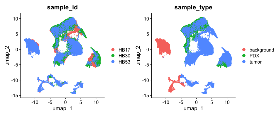
Harmony effectively reduced batch effects across samples, enabling accurate clustering.
4. Clustering and Manual Annotation
We assign biological meaning to clusters using known marker genes (referenced from GeneCards or literature). This allows us to label clusters like “T cells” or “Tumor-like.”
1
2
3
4
5
6
top10 <- FindAllMarkers(harmony_obj, only.pos = TRUE) %>%
  group_by(cluster) %>%
  top_n(10, wt = avg_log2FC)

harmony_obj$celltype <- "unknown"
harmony_obj$celltype[which(Idents(harmony_obj) == "1")] <- "Fetal-like hepatoblastoma"
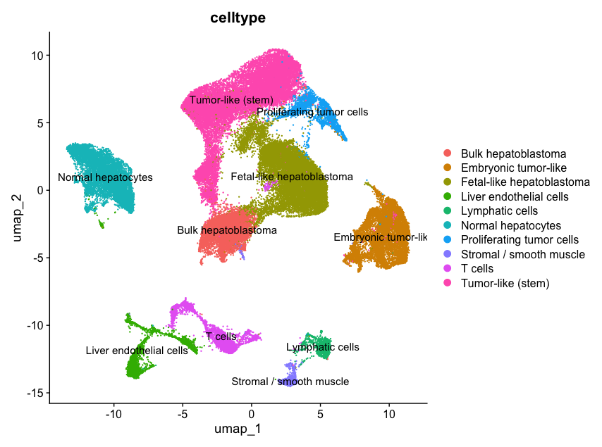
GeneCards was used to interpret marker genes and assign biologically meaningful labels.
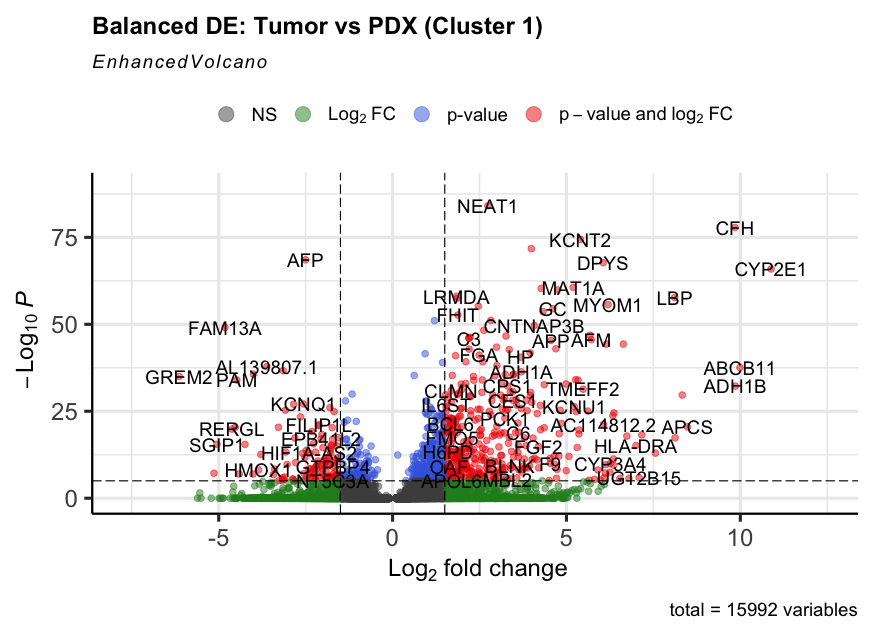
5. Focus: Cluster 1 – Fetal-like Hepatoblastoma
Cluster 1 showed high expression of AFP, SLC22A9, CYP3A7 — matching fetal liver identity. We compared gene expression between tumor and PDX cells to study environmental effects.
1
deg_fetal <- FindMarkers(fetal_like, ident.1 = "tumor", ident.2 = "PDX", logfc.threshold = 0.25)
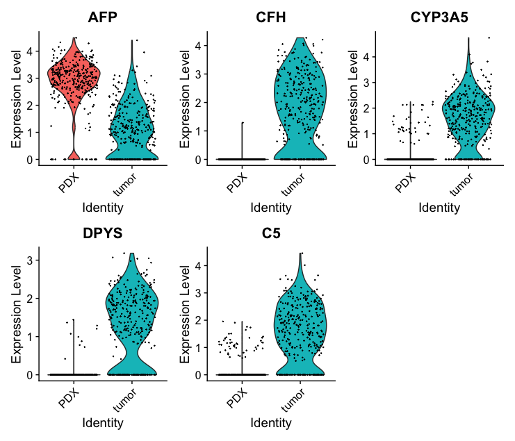
Tumor cells showed higher expression of immune/stress response genes (e.g., CFH, CYP3A5), reflecting their in vivo complexity.
6. Visualization
To explore and communicate gene expression differences, patterns, and marker gene localization across clusters and conditions.
1
2
3
4
DimPlot(harmony_obj, group.by = "celltype", label = TRUE)
DoHeatmap(harmony_obj, features = top10$gene)
EnhancedVolcano(deg_balanced, lab = rownames(deg_balanced),
                x = 'avg_log2FC', y = 'p_val_adj')
Key Insights
- PDX cells retained fetal liver identity; tumor cells diverged under immune pressure
- DGE analysis revealed complement/stress response activation in tumors
- Supports PMID: 34497364: PDXs are cleaner models, but lack complex tumor–host interactions
Conclusion
This project demonstrates a full snRNA-seq analysis pipeline from raw data to biological insight. It combines technical rigor with biological interpretation, showing how tumor context alters transcriptional profiles — and how to build reproducible pipelines using Docker.
Checkout my github repo for this project Github-Link